Adding pie chart in excel

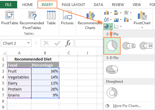
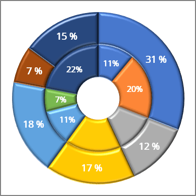
Click on the Insert tab. It is actually a double pie chart which displays the parts of a whole through a main pie while also providing a way to represent.

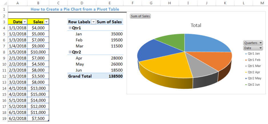
How To Create A Pie Chart From A Pivot Table Excelchat

Click on the drop-down menu of the pie chart from the list of the charts.

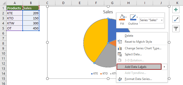
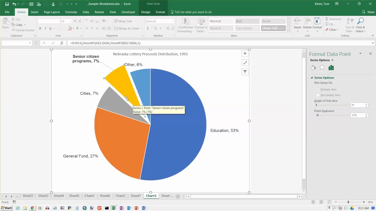
. All pie charts are now. Next choose add data labels again as shown in the following image. Pie-chart gets inserted for the selected values.

Creating a dynamic pie chart using tables We can also. You should find this in the Charts group. To create a pie chart in Excel 2016 you will need to do the following steps.

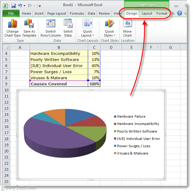
The data labels are added to. To change the chart type of the above chart-. Download and Install a Custom Pie Chart Font Step 2.

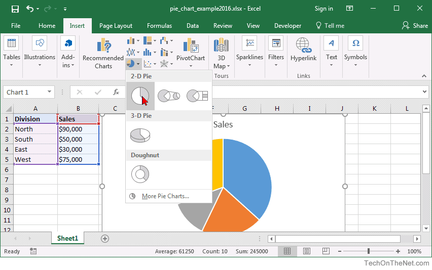
Web Step 1. Highlight the data that you would like to use for the pie chart. Web Excel has a built-in chart type called pie of pie chart.

Click on pie chart in 2D chart. Web Steps to Create a Pie Chart. Select the whole dataset.

Web To create a pie chart in Excel 2016 add your data set to a worksheet and highlight it. Then go to the Insert tab from the Excel Ribbon. Web Click on the first chart and then hold the Ctrl key as you click on each of the other charts to select them all.

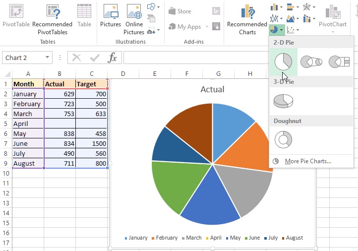
From the dropdown menu that appears select the. Web Bar of Pie Chart in Excel This is similar to the Pie of Pie chart except that a bar constant height replaces the subset pie. Now in the charts group you need to click on the Insert Pie or Doughnut Chart option.

Choose the first option of. Click Format Group Group. Web Go on selecting the pie chart and right clicking then choose Format Data Seriesfrom the context menu see screenshot.

In the charts group Select the pie chart button. In the Chart tab click on the Insert Pie button. Web To insert a Pie Chart follow these steps-Select the range of cells A1B7.

Now select Pie of Pie from that list. Web To create a pie chart- Select the dataset. Web Click on Insert Menu and select the appropriate pie-chart.

Web While your data is selected in Excels ribbon at the top click the Insert tab. Then click the Insert tab and click the dropdown menu next to the image of a. In the Format Data Seriesdialog click the drop down list.

In the Insert tab from the Charts section select the Insert Pie or Doughnut Chart option. Map out the Chart Data Step 3. Right-click the pie chart and expand the add data labels option.

Go to Insert tab. Web Step 1. Web From the Insert tab select the drop down arrow next to Insert Pie or Doughnut Chart.

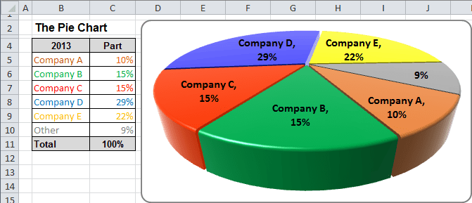
Turn the Custom Values into In-cell Pie Charts Excel In-cell Pie Chart. Below is the Sales Data were taken as reference for.

How To Make A Pie Chart In Excel Using Spreadsheet Data